erDiagram
    state {
        varchar state_code PK
        varchar state_name
    }
    county {
        bigint county_fips PK
        varchar county_name
        varchar state_code FK
    }
    cbsa {
        varchar cbsa_code PK
        varchar cbsa_name
    }
    county_cbsa_code {
        bigint county_fips PK,FK
        varchar cbsa_code PK,FK
    }
    cbsa_rpp {
        varchar cbsa_code PK,FK
        int year PK
        numeric rpp_value
    }
    county_baseline {
        bigint county_fips PK,FK
        int year PK
        numeric population
        numeric median_household_income
        numeric poverty_rate
        numeric unemployment_rate
    }
    county_task_exposure {
        bigint county_fips PK,FK
        int year PK
        numeric routine_cognitive
        numeric routine_manual
        numeric non_routine_cognitive
        numeric non_routine_manual
        numeric routine_cognitive_share "generated"
        numeric routine_manual_share "generated"
        numeric non_routine_cognitive_share "generated"
        numeric non_routine_manual_share "generated"
    }
    county_affordability {
        bigint county_fips PK,FK
        int year PK
        numeric affordability_salary
    }
    state ||--o{ county : contains
    county ||--o{ county_baseline : ""
    county ||--o{ county_task_exposure : ""
    county ||--o{ county_affordability : ""
    county ||--o{ county_cbsa_code : ""
    cbsa ||--o{ county_cbsa_code : ""
    cbsa ||--o{ cbsa_rpp : ""
1 Introduction
Concern about automation is prevalent among American workers. According to Gallup, worries about technology rendering jobs obsolete surged significantly between 2021 and 2023 (Saad 2023). Similarly, the Pew Research Center suggests that Americans expect automation to displace jobs held by others while leaving their own largely unaffected (Smith and Anderson 2017). These surveys capture workers’ beliefs, but they don’t necessarily reflect the actual state of local labor markets. Empirical evidence is lacking to establish whether the concentration of automatable work in a county correlates with the economic conditions faced by its residents. This paper aims to investigate this association.
Autor, Levy, and Murnane (2003) demonstrated that computers replace routine tasks and enhance non-routine tasks, enabling us to identify occupations susceptible to automation. Autor and Dorn (2013) applied this framework to local labor markets, revealing polarization in routine-intensive areas. In these areas, employment grew at both the high and low ends of the wage distribution, while middle-wage employment declined. Acemoglu and Autor (2011) generalized this approach into a model that explains how technology redistributes work across skill groups. This model remains the standard framework for empirical research on automation and labor markets.
None of this work asks what those wages buy where workers live. Outcomes are measured in unadjusted wages and employment shares rather than in local purchasing power. A high wage metropolitan area and a low wage rural county can therefore appear vastly different in dollar terms even when the goods those wages buy are comparable. The unit of analysis is also the commuting zone, which averages over the variation across the counties it contains. Neither feature is a flaw in the earlier studies, which were designed for different questions. Both limit what they can say about county level affordability.
This study asks how the automatability of local jobs relates to county affordability, and whether that relationship holds once poverty and unemployment are accounted for. We build a county by year panel covering 2008 to 2023, excluding 2020, from datasets published by federal agencies. Each county year is summarized by four task group values: routine cognitive, routine manual, non routine cognitive, and non routine manual. These follow the task framework of Autor, Levy, and Murnane (2003) and the occupation taxonomy of Autor and Dorn (2013). The outcome is an affordability salary in dollars, defined as county median household income divided by the local price level from the BEA Regional Price Parities.
We first estimate a panel regression with year indicators and county clustered standard errors, which gives an interpretable estimate of the association. We then check that specification with residual plots, QQ plots, and variance inflation factors. Finally we fit random forest and neural network models to capture structure the linear model leaves behind. Model complexity increases only where diagnostics indicate the simpler specification is insufficient.
2 Background and Related Work
3 Data
3.1 Data collection
Data for this analysis come from five datasets published by three U.S. federal agencies. Each was retrieved through an agency API or bulk file download and loaded into a PostgreSQL database. Table 1 reports each source, record counts, and the variables it supplies.
| Source | Records retrieved | Variables supplied | Warehouse table |
|---|---|---|---|
| Census SAIPE | 50,283 | median household income, poverty rate | county_baseline |
| BEA Regional Price Parities | 884 | county price level relative to the national average | cbsa_rpp |
| Census CBSA delineation | 387 | county to metropolitan area crosswalk | cbsa |
| ACS 1 year estimates | 15,690 | population, occupational employment by category | county_baseline, county_task_exposure |
| BLS LAUS | 88,004 | unemployment rate | county_baseline |
The five sources arrive at two levels of observation: county by year, and metropolitan area. The pipeline transforms each to a common county by year grain, and county FIPS code and year together serve as the join key across the warehouse. Regional Price Parities require one extra step. BEA publishes them at the metropolitan area level, so counties are linked to their metropolitan area through the Census CBSA delineation file before joining.
The study period spans 2008 to 2023, excluding 2020. ACS suspended its 1 year estimates that year following COVID related disruptions to data collection. Because those estimates supply the occupational employment counts underlying the task group values, the task groups cannot be constructed for 2020. The 3,156 counties in the Census county reference file observed over fifteen years yield 47,340 potential county year observations.
3.2 Measuring task structure
Following the task framework introduced in Section 2, each of the broad occupational categories published in ACS 1 year estimates is assigned to one of four task groups: routine cognitive, routine manual, non routine cognitive, and non routine manual. The Census categories carry no such labels, so the assignment follows the classification logic of Autor and Dorn (2013): clerical and sales work as routine cognitive, production and construction work as routine manual, managerial, professional and technical work as non routine cognitive, and service work as non routine manual. For each county and year, the task group totals are the employment sums across the categories assigned to each group, shown in Equation 1.
\[ T_{g,c,t} = \sum_{o \in g} E_{o,c,t} \tag{1}\]
Here \(E_{o,c,t}\) is employment in occupational category \(o\) in county \(c\) during year \(t\), and the sum runs over the categories assigned to group \(g\). The four totals are then divided by their sum, as in Equation 2, so that each county year is described by four values on a zero to one scale that sum to one.
\[ G_{g,c,t} = \frac{T_{g,c,t}}{\sum_{g'} T_{g',c,t}} \tag{2}\]
Normalizing by the four group total converts employment counts into a composition, so counties of very different sizes are described on a common scale and the quantity of interest is the relative mix of work rather than its volume. The implications for estimation are reported in Section 4.
Retaining four separate groups, rather than collapsing them into a single routine intensity index, preserves a distinction that a composite measure erases. Under one index, a county shifting away from clerical work and a county shifting away from assembly work look identical.
3.3 Measuring affordability
The outcome variable is affordability salary, defined in Equation 3 as county median household income, from the Census SAIPE program, divided by the local Regional Price Parity. BEA publishes parities as an index with the national average set to 100, so dividing by 100 converts the index into a price multiplier.
\[ A_{c,t} = \frac{\text{Median household income}_{c,t}}{\text{RPP}_{c,t} / 100} \tag{3}\]
A county with a median household income of $60,000 and a price parity of 120 has an affordability salary of $50,000, meaning local income buys what $50,000 would buy at national average prices. Stated this way, income is comparable across counties, since a given figure purchases roughly the same bundle wherever it appears.
The adjustment is spatial rather than temporal. Regional Price Parities correct for price differences across places but not across years, so affordability salary is not deflated to a constant base year. National price movement over the study period is absorbed by the year indicators in the regression rather than by the variable itself.
Counties outside any metropolitan area have no published parity of their own and take their state parity instead. Within the analytical panel, 45.5 percent of county year rows use a metropolitan parity and 54.5 percent use the state fallback. This is a substantive limitation, since a single state level price index is applied to counties whose actual price levels differ, and a majority of panel rows carry it. The counties involved are above the 65,000 population threshold but predominantly outside metropolitan statistical areas, where BEA publishes no local parity.
3.4 Control variables
Three baseline county conditions enter the models as controls. Unemployment rate comes from BLS LAUS and poverty rate from the Census SAIPE program, both measured in percentage points. Total population comes from ACS 1 year estimates and enters the models in logs. Unemployment and poverty capture labor market slack and material hardship that would otherwise be attributed to task structure. Population accounts for scale differences across counties, which range from the ACS publication threshold of 65,000 to the roughly 10.2 million residents of Los Angeles County.
3.5 Storage and organization
Data are stored in PostgreSQL across two databases that serve different purposes.
The first is a data lake of roughly 41 tables holding raw retrievals and intermediate results, deliberately left unnormalized. Its purpose is traceability. Any figure in this report can be traced back to the records it came from, and any processing step can be rerun without returning to an agency API, including retrievals for analysis branches later scoped out.
The second is the analytical warehouse of eleven tables, whose analytical core is in third normal form. All cleaning occurs upstream, so the warehouse is effectively read only from the perspective of the analysis. Figure 1 shows the seven tables the analysis reads; a population staging table, a compatibility view, and an employment composition table retained from an earlier analysis branch are omitted.
The schema centers on a county table keyed by FIPS code, with state as a reference table. Three fact tables join to county on FIPS code and year. county_baseline holds population, median household income, poverty rate and unemployment rate, county_task_exposure holds the four task group totals from Equation 1, and county_affordability holds the outcome variable. The normalized values from Equation 2 are not computed in analysis code but stored as generated columns, which the database derives from the four totals on every write. The equation is enforced in the schema itself, so no analysis can read a stale or inconsistently normalized value.
Price parities require a separate path. Metropolitan membership is kept out of the county table and in the county_cbsa_code junction table, so counties outside any metropolitan area carry no null CBSA fields, and the crosswalk stands alone as its own fact. From there cbsa connects to cbsa_rpp. Storing parities at the CBSA level reflects the level at which BEA measures them and avoids repeating a single value across every county in a metropolitan area.
3.6 The analytical dataset
The 47,340 potential county year observations described above are the set of records the county table supports, not the set the models estimate on. Two filters reduce it.
Task group coverage is the binding constraint. The occupational employment counts that build the four task groups come from ACS 1 year estimates, which the Census Bureau publishes only for areas with populations above 65,000. Counties below that threshold have no occupational estimates in any year, so no task groups can be constructed for them. This removes 2,308 of the 3,156 counties outright and leaves 12,087 county year observations across 848 counties.
Requiring non missing controls removes a further 104 observations. Every one of the 104 is missing an unemployment rate, giving BLS LAUS a coverage rate of 99.1 percent across the retained counties. Population, median household income and poverty rate are complete. The estimation sample is therefore 11,983 county year observations, and all models reported in Section 4 and Section 5 fit on these same rows.
The population threshold shapes what the results can describe. The 848 retained counties hold the large majority of the United States population but a minority of its counties, and they are more metropolitan, more populous and more economically diverse than those dropped. Rural counties are underrepresented as a direct consequence. Findings should be read as applying to counties above 65,000 residents rather than to counties in general. Section 6 returns to this limitation and to one approach for addressing it in future work.
4 Analysis
4.1 Panel regression
The four task group values described in Equation 2 sum to one, so all four cannot enter a regression together. One serves as the reference category, and we use non routine cognitive. Each remaining coefficient represents the change in affordability salary associated with a shift out of non routine cognitive work and into that group, holding the controls fixed. Each coefficient is a comparison against the reference category. The group values are measured on a zero to one scale. Per percentage point figures reported later therefore divide the estimated coefficients by 100.
Normalizing the four totals by their sum, as Section 3 describes, also resolves a collinearity issue. Left unresolved, that issue would render these coefficients unusable. The unnormalized totals in Equation 1 exhibit variance inflation factors ranging from 13 to 27. All four are employment counts, so they scale together with county size. Dividing by the four group sum removes this common scale and reduces the variance inflation factors to approximately 1.
Year indicators capture conditions common to all counties within a year. These include the 2008 recession, the recovery through the 2010s, and the price movement that affordability salary does not itself account for. Standard errors are clustered by county, because repeated observations of the same county across fifteen years are not independent draws.
4.2 Validation before modeling
Before making any estimations, we ensure that the data support the chosen methods. We examine the distributions of the four task groups and the affordability salary to identify any skewness or outliers. Additionally, we verify that the county-year coverage is consistent across the retained panel. Furthermore, we check for any overlap between task groups to ensure that no two groups effectively carry the same information. Figure Figure 2 provides visual representations of the distributions.
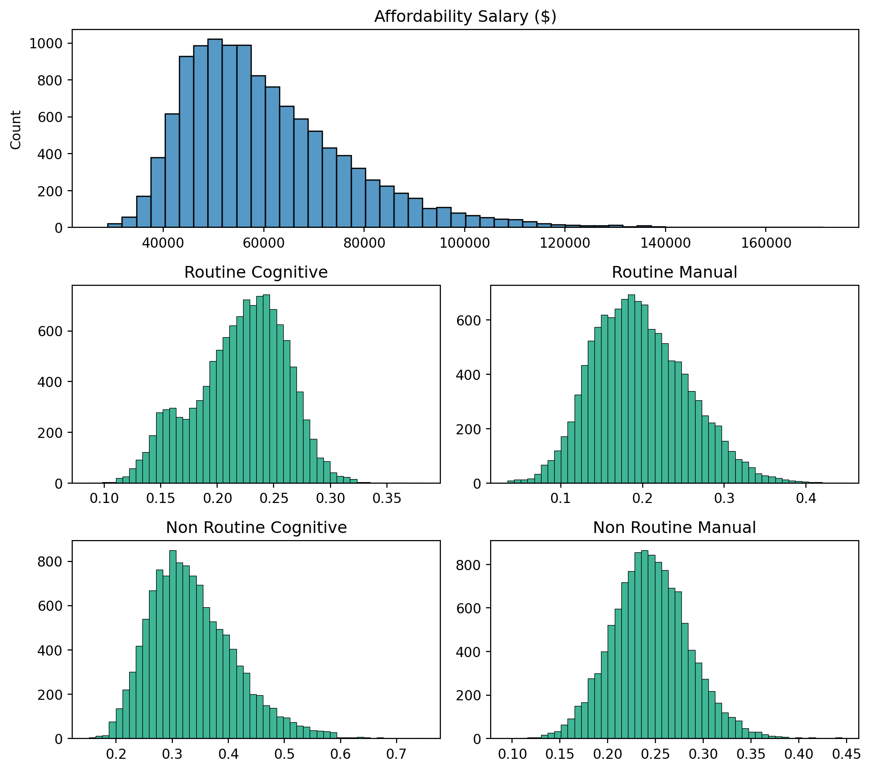
Affordability salaries are right-skewed, with a skewness of 1.17. The center of the distribution is located near $57,000, and a long tail of high-paying counties extends above it. This skewness is why the diagnostics below focus on the extremes of the distribution.
4.3 Specification diagnostics
A linear model assumes a constant rate of association across the data range and symmetrical, evenly distributed errors around the fit. We verify these assumptions using three diagnostics: residuals plotted against fitted values, a QQ plot of the residuals, and variance inflation factors. Figure 3 illustrates the first two diagnostics, pinpointing the failure directly. The smoothed residual line deviates from zero, indicating a non-linear relationship. The vertical spread of residuals increases with fitted values. The model underestimates both the least and most affordable counties while fitting the middle well. Additionally, the QQ plot deviates from normality in the upper tail, suggesting a residual skew of 1.02.
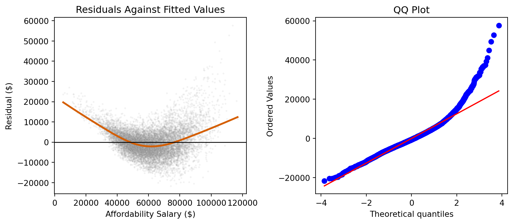
The level model still provides the interpretable estimates we report. Additionally, its own diagnostics demonstrate that the data possess a structure that a straight line in dollars cannot adequately represent. Binned means plots in Section 5 illustrate the underprediction in dollar terms, with approximately $8,000 to $9,000 of underprediction at each tail.
4.4 Log respecification
Underprediction at both extremes is a hallmark of a multiplicative process that is fitted on an additive scale. The factors influencing affordability operate proportionally, resulting in a more significant impact on a high-affordability county compared to a low-affordability one when a similar change occurs in an input variable. By converting the proportional effects into the additive form assumed by linear models, we refit the same specification on log affordability salary. Consequently, the diagnostics respond accordingly, as demonstrated by Figure 4. The residual skew decreases from 1.02 to 0.09, and the spread becomes relatively constant across the fitted range. The QQ plot also straightens through most of its range. The log linear fit serves as the baseline for evaluating the flexible models presented in the subsequent section.
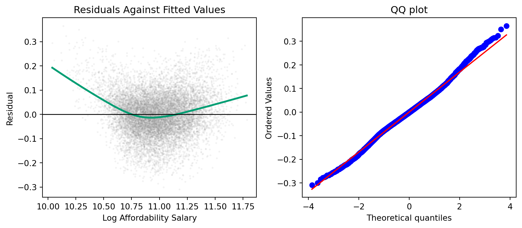
The smoothed residual line doesn’t lie perfectly flat even after the transformation. The remaining deviations are structured in a way that a single global transformation cannot absorb, most likely due to interactions among the inputs. These deviations motivate the increase in model complexity.
4.5 Variance decomposition
Affordability, salary, and task groups vary both across counties and within a county over time. These variations have different implications. The two manual groups show almost complete variation between counties, with only 10-25% variation within a county on the corrected window. This makes the associated affordability differences more durable rather than temporary. Routine cognitive is the only group with genuine within-county movement, with nearly half of its variation on the corrected window.
The Census occupation coding change between 2009 and 2010, as described in Section 3, inflates apparent within-county variation for the routine cognitive group. This is due to the way the source data were coded, not a property of the counties. Therefore, we repeat the main estimates on a panel restricted to 2010 onward and additionally on pre-pandemic (2010-2019) and post-pandemic (2021-2023) windows. Coefficient stability across these windows is reported in Section 5, along with the between- versus within-county exhibits that support the claim of persistence.
4.6 Machine learning models
4.7 wrap up summary [tk]
5 Results
5.1 Where affordability is strained
5.2 Task groups and affordability
The panel regression returns a negative association between routine intensive work and affordability salary that holds after controls. A one percentage point shift toward non routine manual work is associated with roughly $1,041 less in affordability salary [TK: confirm sign, magnitude, and standard error against the current model output, and state which task group carries the largest coefficient].
?@fig-coefplot shows each task group’s coefficient with its confidence interval, non routine cognitive as the reference.
The associations survive the addition of poverty rate and the other baseline controls, so the task groups are not standing in for poverty. ?@fig-coefcompare puts the coefficients before and after controls side by side.
5.3 Nonlinearity
The RESET test rejects the linear specification [TK: statistic and p value], and ?@fig-binned shows why. Binned means of affordability salary across the range of routine cognitive work rise and then fall rather than tracking a straight line.
?@fig-modelcomp compares held out performance across specifications. The random forest reaches a test R² of 0.840 against 0.610 for ordinary least squares, and the neural network 0.739 [TK: confirm all four figures against the current run]. The gap is evidence that the relationship has curvature the linear model cannot represent, which is the same conclusion the RESET test reaches by a different route.
5.4 What matters most
Poverty rate is the strongest single feature in the random forest, by a wide margin (?@fig-importance). Task groups follow, with routine cognitive ranked highest among them. This ordering is consistent with the regression: poverty carries most of the explanatory weight, and the task groups add to it rather than substituting for it.
5.5 Stability over time
A county’s task mix moves very little across the fifteen year panel [TK: quantify]. This matters for interpretation. Because the mix is close to a fixed characteristic of place, the affordability differences associated with it do not fade, and they are not something residents can be expected to move out from under.
5.6 Robustness
Restricting the panel to 2010 onward, which removes the occupation coding change described in Section 3, leaves the main associations intact [TK: report the restricted estimates].
6 Conclusions
6.1 Summary
We asked whether counties with more automatable work are less affordable for the people who live in them. Building a county by year panel from eight federal sources, summarizing each county’s work by four task groups, and measuring affordability as median household income adjusted for local prices, we find that the answer is yes and that the relationship holds once poverty and unemployment are accounted for. Poverty is by a wide margin the strongest single correlate of county affordability. The task mix is a smaller but separate one.
6.2 What this adds
Two patterns are worth stating plainly before the broader claim. Poverty is the strongest single correlate of county affordability, but the task mix relates to affordability independently of it. And neither relationship is a straight line: routine cognitive work shows a rise then fall pattern, and poverty’s association is steepest at low levels and flattens at high ones.
The task framework has been applied to wages and to employment composition, mostly at the national or commuting zone level. Applying it to a cost adjusted outcome at the county level changes what the measure describes: not what work pays, but what that pay buys where it is earned. Two findings follow from that shift. The association is present after controlling for local economic distress, so it is not poverty in different clothing. And it is not linear, which the RESET test establishes and the flexible models exploit, so studies that assume a straight line relationship between task composition and local outcomes are leaving structure on the table.
The finding lands on people through place. Residents of routine work counties see their incomes buy systematically less, and because a county’s task mix barely moves across fifteen years, the difference is built into where they live rather than something individual effort resolves. Three groups can act on that. Economic development agencies deciding where workforce training goes, since the task mix separates structurally exposed counties from those in a temporary downturn. Policymakers and planners designing cost of living responses, since these gaps will not close on their own. And researchers extending the framework, since both the county level link and its nonlinear shape point past existing national wage studies.
6.3 Limitations
The results are associational. Counties are not assigned their mix of work, and nothing in this design isolates a causal channel, so we cannot say that automatable work makes a place less affordable, only that the two move together.
The four task groups are parts of a whole and sum to one, so one had to serve as a reference category. Every coefficient is read relative to non routine cognitive work rather than in isolation.
Coverage is the sharpest constraint. Task group values exist for 12,087 of the 47,340 county year combinations in the frame, and dropping the 104 rows missing an unemployment rate leaves 11,983 for estimation across 848 counties. The counties that fall out are small ones, below the population threshold at which the American Community Survey publishes one year occupational estimates, so the panel describes metropolitan and larger non metropolitan counties rather than the country.
Regional Price Parities are published for metropolitan areas, so counties outside one take their state value. Roughly 55 percent of county year rows use that fallback, which applies a single price index to counties whose actual price levels differ, and it falls disproportionately on rural places.
2020 is excluded because the American Community Survey did not release one year estimates for it. The 2009 to 2010 occupation coding change is a source artifact that inflates measured within county variance for routine cognitive work; restricting to 2010 onward leaves the conclusions unchanged.
The machine learning results rest on a single train and test split [TK: replace with cross validation if time allows].
6.4 Ethical considerations
All data are public county level aggregates with no individual records, so no person can be identified. Two harms are worth naming. Labeling counties as exposed or stuck could stigmatize them or steer investment away from the places that need it. And reading the association as causal could motivate policy that tries to reshape a county’s mix of work in the expectation that affordability follows, which this study does not support.
6.5 Future directions
Two extensions would address the limitations above directly.
The coverage gap could be narrowed with satellite imagery. Jean et al. (2016) estimate local economic conditions from daytime and nighttime imagery where survey data are thin, an approach that could recover the small counties this panel excludes and allow the affordability pattern to be retested on them.
Finer grained labor data would move the work closer to a causal claim. Splitting the task mix by worker education and status would separate the effect of workforce composition from the effect of the task mix itself, which the current design cannot disentangle.
6.6 Conclusion
[TK: the closing paragraph. Zelner’s fourth move, the one that ties it together. What does it all mean, why does it matter, what sticks with the reader. This is the place to be a little more opinionated. Draft line to work from: poverty remains the strongest correlate of county affordability, but the mix of work a county holds is a separate pressure on top of it, and poverty and unemployment statistics alone do not capture the full picture of affordability risk.]
7 References
Acemoglu, Daron, and David Autor. 2011. “Skills, Tasks and Technologies: Implications for Employment and Earnings.” In Handbook of Labor Economics, edited by David Card and Orley Ashenfelter, 4:1043–1171. Elsevier. https://doi.org/10.1016/S0169-7218(11)02410-5.
Autor, David H., and David Dorn. 2013. “The Growth of Low-Skill Service Jobs and the Polarization of the US Labor Market.” American Economic Review 103 (5): 1553–97. https://doi.org/10.1257/aer.103.5.1553.
Autor, David H., Frank Levy, and Richard J. Murnane. 2003. “The Skill Content of Recent Technological Change: An Empirical Exploration.” The Quarterly Journal of Economics 118 (4): 1279–1333. https://doi.org/10.1162/003355303322552801.
Jean, Neal, Marshall Burke, Michael Xie, W. Matthew Davis, David B. Lobell, and Stefano Ermon. 2016. “Combining Satellite Imagery and Machine Learning to Predict Poverty.” Science 353 (6301): 790–94. https://doi.org/10.1126/science.aaf7894.
Saad, Lydia. 2023. “More U.S. Workers Fear Technology Making Their Jobs Obsolete.” Gallup. https://news.gallup.com/poll/510551/workers-fear-technology-making-jobs-obsolete.aspx.
Smith, Aaron, and Monica Anderson. 2017. “Automation in Everyday Life.” Pew Research Center. https://www.pewresearch.org/internet/2017/10/04/automation-in-everyday-life/.