Introduction
Rapid legalization of gambling across the United States and the rise of app-based and online betting platforms has propelled sports betting into a multi-billion-dollar industry. This transformation has introduced new forms of entertainment, economic opportunity, and media attention for athletes, but it has also sparked critical questions about who participates in this growing industry and why. Specifically, how are patterns of sports betting participation distributed across socioeconomic groups? The new age of sports betting has introduced additional gambling risks. Because of these reasons, we seek to answer: How do the socioeconomic factors: education and income, correlate with sports betting handle at the state level?
Our hypothesis is that groups of lower socioeconomic status, with particular regards to income and education, would see higher rates of sports betting participation. Historically, gambling in general has been associated with lower-income and less-educated households. However, with sports betting being such a new venture in the gambling world, it is not widely associated with these socioeconomic trends yet. However, if these groups are in fact participating at a higher rate than others of higher socioeconomic standing, it raises concerns. For many individuals, gambling may reflect not recreational entertainment, but economic desperation, misinformed optimism, or a perceived path to financial mobility. In such contexts, the consequences of betting can deepen cycles of financial instability. At the same time, education levels may influence individuals’ understanding of risk, probability, and long-term outcomes, potentially creating an equity gap in financial decision-making and loss aversion.
Relevant Vocabulary
Gambling: Gambling is the act of wagering something of value (usually money) on an event with an uncertain outcome, primarily for the purpose of winning additional money or material goods. It includes a wide range of activities such as lotteries, casino games, poker, and sports betting.
Sports Betting: Sports betting is a specific form of gambling in which individuals place wagers on the outcomes of sporting events. While sports betting can be done in person, with the recent popularity of sports betting mobile apps, it has become one of the fastest-growing sectors of the gambling industry.
Handle: In the context of gambling, handle refers to the total amount of money wagered by bettors, regardless of whether the bets are won or lost. For example, a state’s monthly sports betting handle reflects the gross volume of bets placed, not the revenue retained by operators or the winnings paid out.
Background
Existing research on gambling behavior has long highlighted disparities in participation and harm across socioeconomic lines. Individuals with lower income and education levels are more likely to engage in gambling activities and to experience gambling-related harm. These patterns suggest that gambling is often more than a recreational activity among vulnerable populations, but rather means for perceived financial gain; driven by economic hardship or limited financial literacy. ((Williams, Volberg, and Stevens 2011), (Welte et al. 2004))
Much of the existing literature focuses on traditional forms of gambling, such as casinos, lotteries, or scratch tickets, rather than sports betting, which has recently evolved due to mobile technologies and policy shifts. The legalization of sports betting across more than 30 U.S. states, coupled with app-based betting platforms, has introduced a new gambling ecosystem. Initial studies suggest that online sports bettors tend to skew younger and more male, and may differ in behavior and motivations from traditional gamblers. For example, gambling among this group is considered more of a social activity, which could introduce peer pressure or performative actions. (Volberg, Nysse-Carris, and Gerstein 2010)
Because of the developing nature of this sector, studies have not examined how socioeconomic factors such as income or education level correlate to participation in sports betting to the same degree as studies on traditional gambling. This gap in the literature is significant given the rapid expansion of the sports betting industry and its integration into everyday digital life.
Our study seeks to address this gap by examining correlations between sports betting fiscal data and state-level demographics, particularly educational attainment and income. By focusing on macro-level data across states where sports betting is legalized, we aim to identify whether historical socioeconomic disparities in gambling participation are mirrored in the newer domain of sports betting. If lower socioeconomic status is indeed linked to higher sports betting participation, this would suggest a need for proactive public health messaging and regulatory safeguards tailored to the unique risks of app-based platforms.
Therefore, this study aims to reveal the correlation between sports gambling and socioeconomic factors with the hope to understand the predictors and if warnings or precautionary steps should be taken to prevent adverse effects to certain participants. While we hypothesize a positive correlation between these factors, our real hope is to deepen the understanding of this growing field to protect against misuse of the activity.
Data
With the goal of this project being to investigate the correlation between sports betting rates and education/income trends across U.S. states, we collected and compiled data from multiple sources. The first dataset, titled Online Sports Betting Dataset, was the most straightforward. This data included information about the 31 legalized states in sports betting and was retrieved from https://rg.org/statistics/us. Since the data was not contained in an easily scraped format, we downloaded it manually by switching between the year toggle button to get access to all the publicly available data. In doing this, we were able to gain sports betting data from 26 states as multiple states have sports betting activity through tribal casinos or have only been legalized in the year 2025 so there is not data available yet. Since the process of getting this data was straightforward, it did require any additional cleaning.
In contrast, collecting income and education data from the U.S. Census (covering the years 2018–2023) proved more complex. The range from 2018-2023 was selected because it represents the overlap of available years across our datasets. However, due to the structure of the Census API, each year and state combination was available at a different API endpoint. Additionally, the topic parameter (either income or education) had to be specified separately. This meant that retrieving data for the 31 included states across six years, for two topics, would have required 384 manual downloads and subsequent joins.
To avoid this, we built a web scraper using Docker, Supabase, PostgreSQL, and Beekeeper Studio. From the Census, we were able to grab a variable identifier called GeoID which are numeric codes that uniquely identify all geographical areas for which the Census Bureau. In our case, this contains all the ids that identify the states we want to scrape for.
The scraper looped through the year and GeoID values in the API URL to pull each required combination in one run. However, we opted to run the scraper twice, once for income and once for education, manually replacing the topic ID in the scraper.py file between runs, rather than building the scraper to run both topics. The logic behind this decision was that it was simpler to change one number in the scraper.py file and run it a second time, than create a scraper that switched which table it was dumping into halfway through, since storing education and income in two individual tables was better for the planned analysis.
To automate this process and manage dependencies across our local devices, we used Docker. Docker allowed us to contain our scraping environment so that all required libraries, API keys, and files could be packaged into a single reproducible environment. This ensured that the scraper would run identically regardless of the local setup and all us to deploy the scraper in a controlled environment,
For data storage, we used Supabase which is an open-source backend service platform that provides a hosted PostgreSQL database along with API keys and file storage features. This acted as a cloud layer that hosted our PostgreSQL instance, making it accessible to both members of our team without having to manage database infrastructure ourselves. Supabase connects directly from our local tools for easy querying and inspection. We then stored all the scraped data in Beekeeper to clean and work with.
Once scraped, we employed SQL to clean and normalize the raw JSON responses into a table format. We scaled down our data by selecting only the variables relevant to our analysis, choosing only columns relating to the full distribution of a state or for the main households that covers a majority of the households data and how it was organized. These choices were made preemptively to avoid overflowing data and give us a narrowed scope that would help give a more coherent explanation of the data. This process resulted in three final tables: the sports betting dataset, the cleaned income dataset, and the cleaned education dataset, all of which were stored on local systems for the remainder of the project.
For each dataset, we performed several operations to ensure consistency across columns and formats. We first conducted basic data cleaning and wrangling where the column values and names were altered to be consistent among all the data. The next step was finding a common variable among our three datasets as sports betting had a different column name containing states. Geoid and year became our primary identifiers across our sports betting, cleaned income, and cleaned education datasets. This also allowed for simple screening for duplicates among the tables that may have the same geoid and year, and we were able to filter those out quickly. There was only one duplicate row found that was a result of a faulty run on our part but it was quickly removed. We created a location table that showed the corresponding state name to each geoID, which worked as a connection between all tables. After that we normalized the data structure in 3rd Normal Form to allow us the best structure for our planned analysis.
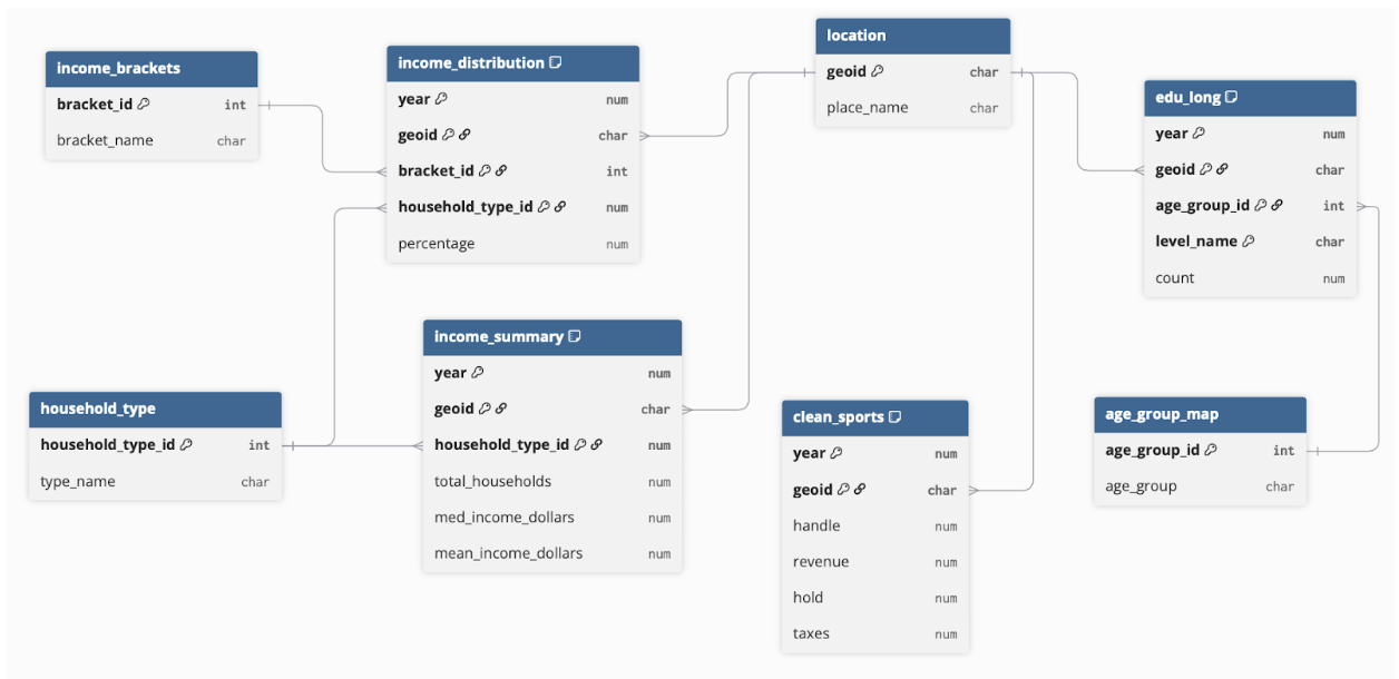
As seen in Figure 1, to support analysis of the relationship between sports betting activity and socioeconomic trends across U.S. states, the data was structured into a schema that separates income, education, and betting metrics into connected tables to facilitate flexible joins. Geoid and year serve as foreign keys linking all domain-specific tables (income, education, and sports betting) to the central location table that maps each geoid to a state-level place_name. Income data is organized into two fact tables. The income_distribution table captures the percentage of households within each income bracket and household type, while the income_summary table provides metrics such as total households, median income, and mean income by household type. These reference the income_brackets and household_type dimension tables for consistency. Education data is stored in the edu_long table, which reports the number of individuals by education level and age group. It joins the age_group_map table to normalize age categories. Sports betting data is stored in clean_sports, which contains metrics such as handle, revenue, hold, and taxes. This table integrates with the rest of the schema via shared identifiers. This structure allows for efficient querying as we explore the research question.
Results
Due to the presence of two socioeconomic predictors in this analysis, a two pronged approach was used to evaluate each predictors impact on sports betting individually. Because of the limited knowledge of known sports-betting motivators, we felt this was the best approach considering no direct correlation between the combination of these variables and sports betting has been made to our knowledge. We evaluated the connections between education and income’s individual relationships with sports betting indicators to see the true results.
Statistical Thinking
To explore the potential correlation between sports betting activity and educational attainment, we used a multiple linear regression model. Statistical thinking in this context allowed us to distill sports betting into a model that quantifies relationships between education level and betting activity, while also accounting for uncertainty. Naturally, this was the first step of our analysis and was primarily conducted as a validation to move forward with the planned direction of analysis.
Our education model examined the relationship between the percentage of a state’s population at various education levels and the per resident sports betting handle (“hand_per_capita”) using state-level data. The model included five predictor variables: percent of adults without a high school degree hs_no_grad_pct, high school graduates hs_grad_pct, associate degree holders ass_pct, bachelor’s degree holders bach_pct, and graduate or professional degree holders grad_or_prof_pct. Because we were working with fiscal data and population counts, if we did not scale it using percentages the model would have simply correlated higher populations with higher total handle.
Our linear model achieved a p-value of 6.642e-06 when considering all five levels of degree attainment. This shows a statistically significant correlation between different levels of degree attainment and handle per resident. Notably, the most influential variable was the bachelor’s degree percentage, indicating that advanced secondary education could affect state level sports betting activity. This modeling approach was appropriate for our research question because we sought to understand not just the presence of a relationship, but the strength and direction of influence that each educational level may exert on sports betting participation, which directed later stages of our research as it revealed what areas in which we should focus.
Linear regression allowed us to estimate how each education category contributes to variations in betting revenue. The results suggest that among all educational categories, the proportion of bachelor’s degree holders (bach_pct) had a statistically significant relationship with sports betting revenue. We will discuss that this means in terms of handling per person in the next section. (Machine Learning) Other education categories, including high school dropouts and associate degree holders, showed no statistically significant effects on their own.
While the model showed potential correlation, it doesn’t necessarily mean it correlated in favor of our hypothesis, so the next step for the education analysis was to further evaluate in what way these variables interacted with one another, which we evaluate starting in the next section. The model yielded a modest R-squared value of 0.2907, indicating that approximately 29.07% of the variance in sports betting revenue per capita can be explained by educational attainment variables. This suggests other factors (such as income) are also influencing participation.
We applied a similar statistical thinking approach to explore the potential correlation between income levels and sports betting activity. Our income model incorporated both household count and income variables, using per-household normalization to avoid misleading conclusions driven by raw scale. Before modeling anything, we conducted a correlation analysis to evaluate the strength of linear relationships between income metrics and sports betting variables (see Figure 2). This preliminary step confirmed strong correlations between total households and both handle and revenue, as well as moderate correlations with income metrics.
Our analysis utilized state-level data and focused on three key predictors: mean income (mean_income_dollars), median income (med_income_dollars), and the total number of households (total_households). We first modeled total sports betting handle as a function of these variables. As shown in Figure 2, the results indicated that all three predictors were relatively correlated. In particular, total households had the strongest relationship, with both revenue and handle suggesting a scaling effect. Mean income and median income had moderate correlation with both handle and revenue as well.
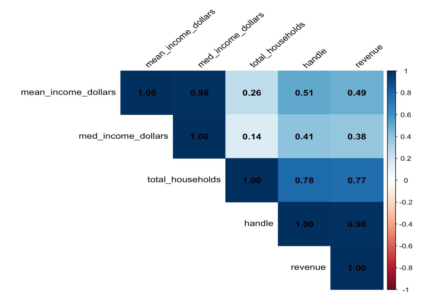
A high mean income coupled with a relatively lower median suggests a skewed distribution with a concentration of wealth among high earners. After some analysis, we found the involvement of the total households variable seems to be skewing our data. To address this issue of population bias, we decided to normalize handle by dividing it by the total number of households, creating the handle_per_household metric. This caused a significant shift in our model’s performance metrics, as shown below:
| Variable | Pre-Normalization | Post-Normalization |
|---|---|---|
| R² | 0.7224 (72.24%) | 0.4027 (40.27%) |
| P-value | 0.00366 | 0.000192 |
Before normalization, our model explained 72% of the variance—but much of this was inflated by population effects. We found that total_households was actually inflating our R² and gave a misleading sense of predictive power. After adjusting for population size, our model explains 40% of the variance and is still highly significant, meaning we’ve removed a key bias while retaining a real relationship. By removing the population size effect, this normalization allowed us to model a true underlying relationship between our variables, making the statistical relationship more clear.
These linear models provided a solid foundation for understanding the direct associations between our variables, but their assumptions of linearity and independence could potentially miss more complex interactions. Taken together, the findings suggest that states with higher mean income levels tend to see greater per-household betting participation, possibly due to increased disposable income or different spending behaviors among higher-income populations.
Conversely, the negative effect of median income may imply that income inequality, or the presence of high earners pulling up the mean, plays a more subtle role in shaping betting habits. This normalization is crucial because raw totals such as total handle are highly sensitive to population differences across states. Without adjustment, larger states would appear to have higher betting activity simply due to scale. By expressing handle on a per-household basis, we focus the analysis on behavioral intensity rather than raw volume, making comparisons across states more meaningful.
These results complement our education analysis by highlighting that not only do demographic factors such as education level relate to sports betting behavior, but so do financial factors. Importantly, both analyses underscore the need to control for population size and distributional effects when modeling large-scale behavioral data such as gambling activity. This leads us to need to use machine learning to further understand these findings from our statistical thinking work.
Machine Learning
As mentioned above, we employed a random forest regression model to understand the relative importance of different education levels in predicting per capita sports betting activity. Machine learning models, particularly methods like random forests, are used for uncovering nonlinear relationships and interactions between variables that standard linear regression might miss. Linear models assume additive, independent relationships and normally distributed residuals; Random Forests handles nonlinear relationships and potential multicollinearity between education categories, which are likely correlated in real-world populations.
Our random forest model was built using the randomForest package in R. The outcome variable was hand_per_cap with the same predictors as our statistical thinking linear model. (Percentages of populations with a certain education level) We trained the model with feature importance analysis, helping us identify which variables contributed most to the prediction of sports betting handle.
From the model output, we observe that the coefficients suggest a strong positive relationship between bachelor’s degree attainment and betting per capita +31.24. These results somewhat mirror those found in our earlier multivariable regression, concluding that bachelor’s degree appears to have an influence on sport betting handle. However, it was revealed that it may not interact with the handle in the way we anticipated. We hypothesised that lower education would correlate with high handle, but this shows the opposite.
This convergence across one parametric model and one non-parametric model makes us confident that our findings are not artifacts of model structure or assumptions. In fact, Random Forest’s showing the same insight boosts our confidence that the relationship is meaningful and not merely coincidental or driven by outliers. These findings give us sufficient motivation to move on to visualizing the specific trends between bachelor’s degree attainment and sports betting handle.
To complement our statistical regression analysis and further examine the relationship between income and sports betting activity, we applied both linear and logistic machine learning models using the caret package in R. These models provided different analytical lenses: regression for predicting a continuous outcome (handle_per_household from sports betting) and classification for distinguishing between “high” and “low” sports betting states based on income-related variables. This dual approach allowed us to evaluate whether income metrics meaningfully predict betting participation, and whether such effects persist across model types.
We began by training a multiple linear regression model, using handle_per_household as the continuous outcome. Predictor variables included mean_income_dollars, med_income_dollars, and total_households. In this model, total_households emerged as a statistically significant positive predictor (p = 0.0025), while both mean and median income had small, non-significant coefficients. This suggests that, at the state level, the number of households is more closely associated with per-household betting activity than income levels themselves. The model’s R² of 0.459 indicates that about 46% of the variance in per-household betting revenue is explained by these predictors, reflecting moderate explanatory power. An actual-versus-predicted plot showed points scattered around the 1:1 reference line, consistent with a model that captures some—but not all—of the variability.
To examine the problem from a classification perspective, we transformed the continuous target into a binary outcome: states were labeled “High” if their handle_per_household exceeded the median, and “Low” otherwise. We then fit a logistic regression model with the same three predictors. The classification model achieved an overall accuracy of 73.2%, substantially higher than the no-information rate of 50.5% (p < 0.00001). Sensitivity (66.7%) and specificity (79.6%) indicated the model performed reasonably well at identifying both high and low betting states. In this case, total_households again emerged as a significant predictor (p = 0.0349), while neither income variable was statistically significant.
Taken together, these models reveal a consistent pattern: household count shows a significant relationship with sports betting participation across both regression and classification frameworks, whereas income variables do not. This likely reflects structural and demographic factors—such as population size, urbanization, or market reach—rather than direct effects of income levels. In contrast to some of our other socioeconomic analyses, these results suggest that income is not a dominant driver of state-level sports betting intensity.
The combination of these models reveals a consistent signal: income is not a particularly strong standalone predictor of sports betting participation, but total household count does show a consistent association. This could be reflecting structural factors like urbanization, market size, or marketing reach rather than income. Importantly, these results contrast with our findings on education, where the relationship with betting was both stronger and more interpretable. These machine learning models together help clarify that while income may play a role, it is not the dominant socioeconomic factor in predicting sports betting activity.
While our statistical thinking and machine learning revealed some potential trends, we wanted to use visual analysis to see where the suspected correlation and negations were, and if we could further prove or disprove our hypothesis.
Data Visualization
Because our study investigates structural socioeconomic predictors of sports betting participation across U.S. states, visualization allowed us to explore spatial and demographic variation that would be obscured in a purely tabular or statistical summary. This was specifically helpful for our research question because of the twenty-six states that were relevant to our analysis. To evaluate education, we employed three types of visual techniques: grouped bar charts, choropleth maps, and bivariate scatterplots with linear models.
This grouped bar chart was created to compare regional averages of sports betting contribution and educational attainment per state. Regional grouping (Midwest, Northeast, South, and West) helped reduce state-level noise and highlight trends across large geographies.
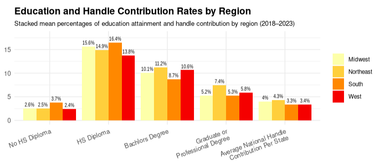
Including education categories side-by-side reveals internal contrasts. And if you point your attention to the bachelors degree and graduate degree groups and compare them to handle contribution, (on the right most side) you can see the progression of increase and decrease between the regions follows the same progression. This is different from the No High School Diploma and High School Diploma columns where there are no clear similarities to the handle contribution. This expands on the trends that we have been seeing; pointing to that higher education correlates with higher sports betting handle state-wide.
To better understand geographic variance, we used choropleth maps to visualize state-level differences in both betting behavior and education attainment. Comparing the handle per capita map (left) with a visualization of advanced degree prevalence (right) allowed us to visually test whether educational attainment is geographically co-located with higher levels of betting activity. We particularly chose to visualize the attainment of a bachelor’s degree or higher based on the results from the models and the previous graphic.
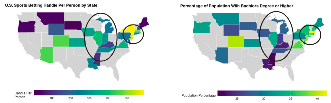
A noticeable feature of this graphic is that the Northeastern region stands out on both maps, high in handle per person and in advanced degree rates. A second area I would like to point your attention to is the midwest and parts of the south, where the progression of education rates and betting handle coincide. While not every state or region have perfect alignment, there are notable similarities between the two maps.
At this point in our education analysis we were seeing strong trends of advanced education correlating with higher handle. So we created two scatterplots with trend lines as a final visual to evaluate this trend.
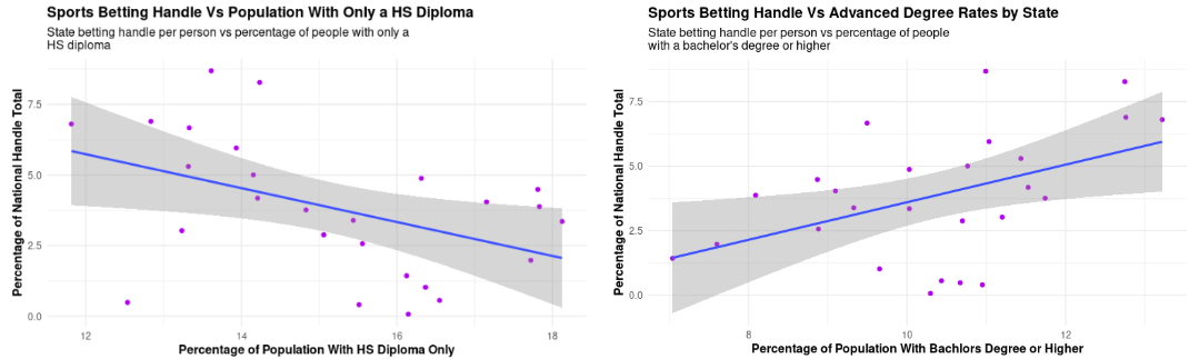
On the left, we see a negative correlation between the percentage of adults with only a high school diploma and their contribution to national handle. On the right, when looking at advanced degree attainment, we observe a positive relationship. While both graphics do have some divergence, there are clear trend lines perpetuating the positive and negative correlations.
Ultimately, these visualizations further debunked our hypothesis, instead, states with higher proportions of individuals with bachelors and graduate degrees appear to accumulate more sports betting handle.
We did a similar approach to explore the relationship between income and sports betting participation across U.S. states. These visual tools helped us examine how both average and low-income populations relate to betting behavior, using a combination of scatterplots and choropleth maps. By incorporating both normalized and disaggregated income measures, we were able to contextualize betting activity within broader socioeconomic landscapes and challenge simplistic assumptions about gambling participation.
To visualize geographic variation in income and betting simultaneously, we employed the use of choropleth maps. The map in Figure 6 displays normalized betting handle_per_household, in relation to percentage of low-income household within each state.
This choropleth map reveals distinct geographical patterns in the relationship between income and betting behavior that are not evident from scatterplots alone. The map highlights two primary regions with a high sports betting handle per household. First, a cluster in the Northeast is characterized by higher-income households and a high handle. Second, a corridor from the West through the Central U.S. shows similar high-volume betting markets, suggesting that this behavior is not confined to a single demographic profile. A particularly notable finding is the cluster of states in the South where a higher percentage of low-income households corresponds with a high handle per household.
This contrasts sharply with the Northeast and suggests that in these specific states, sports betting may represent a significant expenditure for lower-income households. Finally, the map shows that states with a low handle per household are distributed across the country and the income spectrum, with states like Washington categorized as higher-income, low-handle and others like West Virginia as lower-income, low-handle. This demonstrates that a low betting handle is not solely determined by income but is likely influenced by other variables such as state-specific regulations or market maturity.
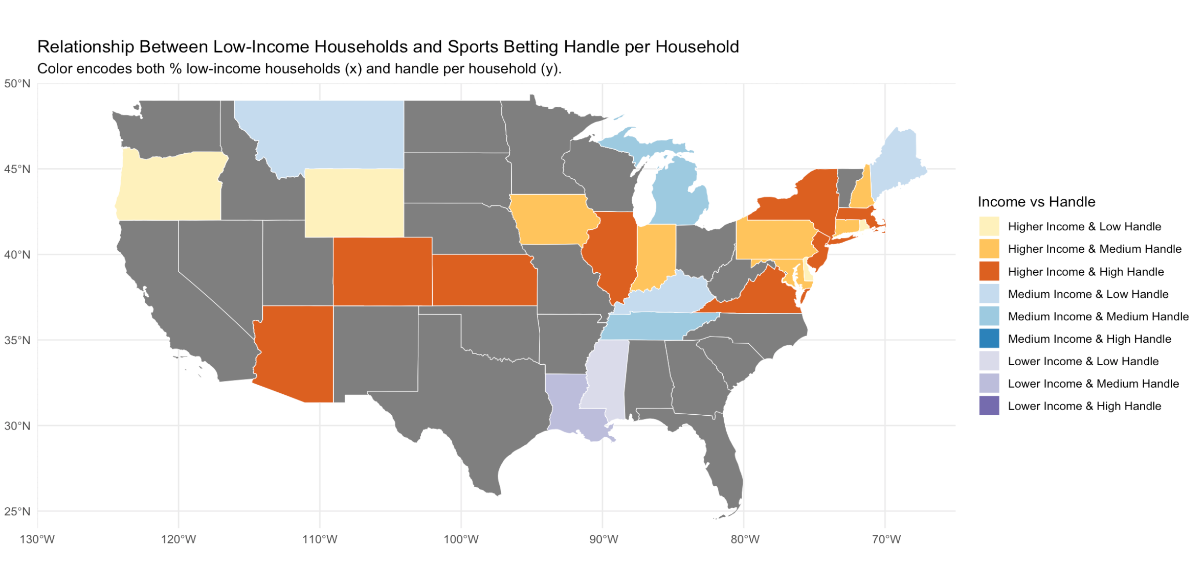
This map shows how income levels and sports betting activity intersect across states. Higher-income states with high betting activity appear in the Northeast, Midwest, and Southwest, while medium-income states generally show lower to moderate betting levels. Lower-income, high-betting states are rare, but the presence of some lower-income states with moderate betting could signal potential vulnerability to gambling-related harm. This map shows that the states with the highest betting activity per household are often not the ones with the highest percentage of low-income households — in fact, many of them fall in higher-income categories. Lower-income, high-betting states are rare, which challenges the traditional belief that gambling is primarily driven by poverty. Instead, the pattern we see here supports our finding that sports betting is more common among affluent, educated, and digitally connected populations — likely driven by greater internet access, cultural normalization, and disposable income.
This finding went against our initial hypothesis that sports betting activity would be most concentrated in states with a higher percentage of low-income households, driven by the theory that gambling serves as a means of seeking economic relief. The distinct visualization of high betting activity in high-income states and the rarity of the opposite challenged this assumption. This observation was a crucial turning point, inspiring us to create a scatterplot to further explore this relationship. By plotting the percentage of low-income households against the handle per household, we could more precisely verify whether this inverse relationship held true across all states or if the regional patterns observed on the map were the result of other confounding variables.
As shown in Figure 7, this scatterplot provided the final confirmation, revealing a clear negative relationship that ultimately negated our initial hypothesis on the income side as well. As the distribution of low-income households increases, betting activity per household tends to decrease. This pattern directly contradicts the traditional view that gambling is driven by poverty. Instead, it aligns with our finding that sports betting participation is higher among more affluent, educated, and digitally connected populations—likely fueled by greater internet access, cultural acceptance, and disposable income. While the overall trend is undeniable, it is worth noting the outliers of Louisiana and Mississippi, which were among the few lower-income states with higher-than-average handle contributions.
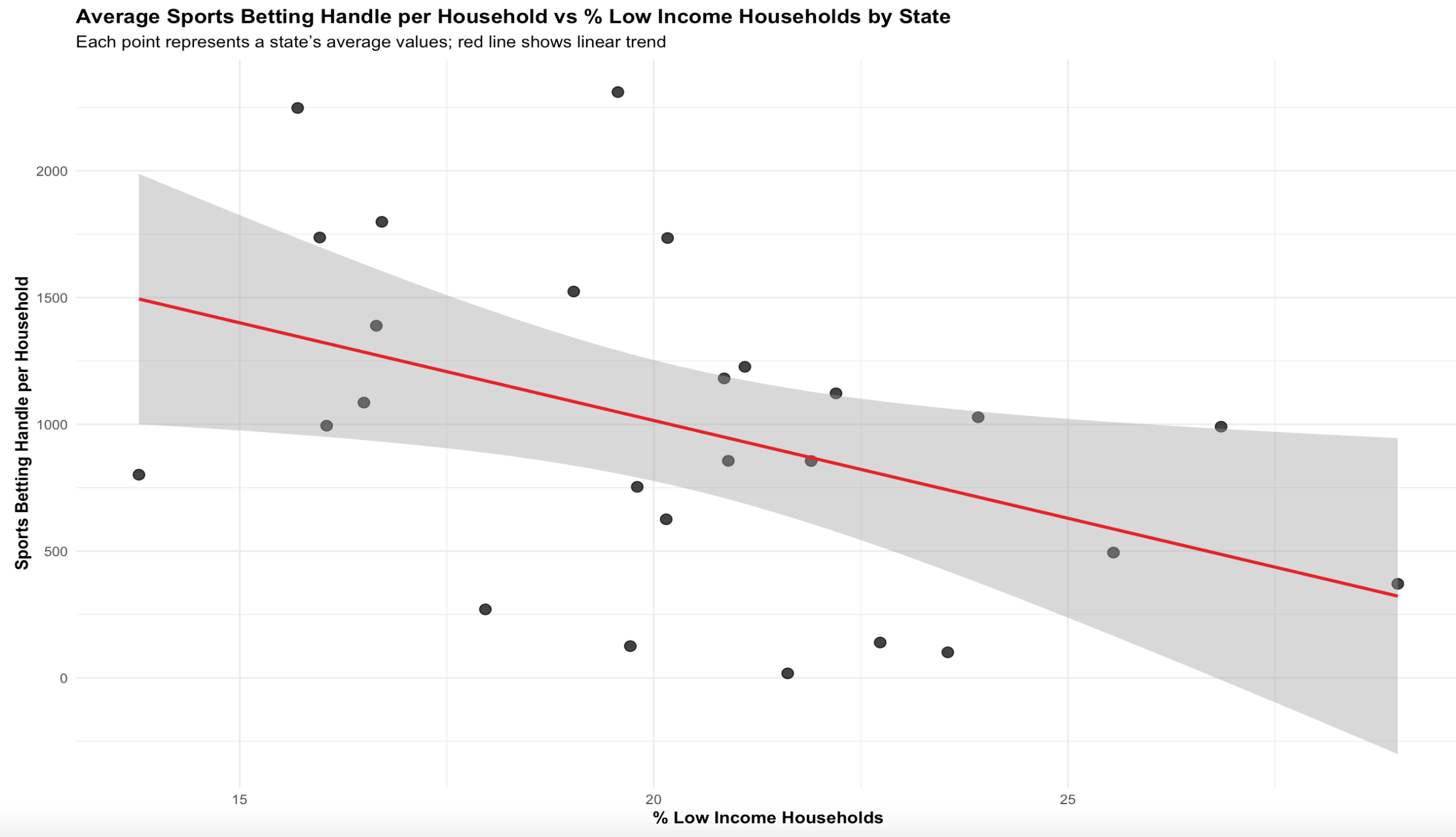
While this may seem counterintuitive to some policy narratives, it aligns with economic theory suggesting that disposable income is a prerequisite for discretionary spending, including gambling. This result challenges the common narrative that sports betting is driven primarily by economic desperation. This indicates instead that participation may be more prominent in higher-income populations with greater discretionary spending capacity.
States with greater proportions of middle- and upper-income brackets often also had higher per capita betting handle, offering yet another lens into how income levels may facilitate or constrain sports betting activity. These visuals suggest that sports betting in the United States is not predominantly driven by poverty, but rather may be a behavior more concentrated among middle- and higher-income earners. This finding directly complicates common assumptions and reveals the value of visualizing normalized and disaggregated income data alongside betting metrics.
Our analysis underscores that betting participation could be shaped less by financial distress and more by access, regulation, opportunity cost, or any other factors often underexplored in blanket narratives about gambling behavior.
Data Ethics
We used publicly available datasets from the U.S. Census and state-reported sports betting metrics. This approach minimized privacy risks, as no personally identifiable information (PII) was collected or processed at any stage of the analysis. Nevertheless, working with demographic and behavioral indicators, such as income, education, and gambling activity, still required caution. Even when data is de-identified, aggregation can lead to the reinforcement of stereotypes or the masking of structural inequities. To mitigate this risk, we chose to analyze only state-level trends, avoiding county- or zip-code-level disaggregation that could disproportionately spotlight or stigmatize smaller or more vulnerable populations; and we encourage future research into this sector to evaluate aggregated data as a precaution as well.
We were careful not to frame our findings in terms of moral judgment or individual responsibility, instead focusing on structural correlations that imply there are populations who might be vulnerable to misuse. If future analysis were to consist of individual-level analysis, findings from that study could open the door to manipulative use of people’s data. For example, if a sports-betting company can predict an individual’s behavior associated with gambling, they can direct specialized ads and notifications to maximize handle from that user. This could lead to financial disturbance in that person’s life, especially if they already struggle with gambling habits.
However, with that recommendation in mind, it is worth noting the potential benefits of individual-level data. If sports betting apps could create a dashboard that presents a user’s habits to the average across the app, it could help the user recognize if their behavior is entering dangerous territory. While this would clearly help sports betting apps maintain a user friendly environment, we would urge nation-wide policy to guide use of this data; limiting the use cases of this data for strictly behavioral health, and prohibiting companies to use it for any form of marketing or targeted promotions for users.
Another ethical concern lies in bias baked into the original data sources. U.S. Census data, while comprehensive, could have limitations in how it categorizes income and education. It may undercount certain populations (especially undocumented individuals, rural residents, and Indigenous communities), which can skew representational accuracy.
Sports betting data, on the other hand, only includes legal, reported activity, ignoring illegal or unregulated markets where participation may also be significant, particularly in states that have not legalized betting. This creates an incomplete picture of the true landscape and potentially biases our conclusions toward the behavior of more affluent, digitally connected populations who are more likely to use app-based platforms.
Our analysis consisted of only 26 states, barely more than half of US states. While we prefaced this in our writing, if it were not properly disclosed it could lead to over-generalized assumptions about U.S. sports betting trends.
Lastly, we would like to recognize how our results could be interpreted, or misinterpreted, in public discourse. Gambling is a socially and politically charged topic, often laden with stigma. Suggesting that certain populations are more likely to gamble can quickly spiral into harmful narratives about irresponsibility or moral failing. Our aim was not to pathologize individuals, but to investigate structural patterns that may reflect underlying disparities in access, education, or economic opportunity. To that end, our findings are not meant to be deterministic conclusions, but rather context for further research, general awareness, or future policies to protect users.
Conclusions
This project set out to investigate whether socioeconomic indicators, specifically education and income, could help explain variations in sports betting participation across U.S. states. Our initial hypothesis, informed by patterns observed in traditional gambling literature, assumed that individuals with lower education and income levels would participate more heavily in sports betting. However, our findings revealed a more nuanced picture. Education emerged as a particularly important factor, though not in the way we expected. Rather than lower educational attainment predicting greater sports betting activity, our analysis identified an increase in sport-betting activities with advanced degree rates, specifically bachelor’s degree attainment as the strongest predictor of increased per capita betting. This suggests that sports betting, especially in its app-based form, may appeal more to college-educated individuals; perhaps due to factors like digital fluency, marketing exposure, cultural normalization, and the increased disposable income most bachelor’s degree holders have, which leads us to the trends we saw in our income section.
While mean income had a modest positive association with betting handle per household, total household count showed stronger predictive value. This may reflect structural factors such as population density rather than individual financial behavior. Contrary to narratives that link gambling primarily to financial desperation, our analysis suggests that disposable income may be more relevant to understanding who participates in legal sports betting. Taken together, these results complicate traditional assumptions about gambling behavior. They show that sports betting, as a modern and heavily marketed phenomenon, interacts with socioeconomic indicators differently than casinos or lotteries have in the past. In particular, lower educational attainment may correlate with lower income and thus less disposable cash.
Ultimately, although we negated our original hypothesis, we believe our findings contribute a valuable dimension to public policy and risk regulation discourse. By identifying education and income as meaningful predictors, we hope to support more targeted and equitable safeguards, ones that recognize the diversity of participation across the socioeconomic spectrum rather than relying on outdated generalizations. Future work on this topic should expand the scope of variables under consideration, perhaps incorporating additional census metrics such as race, age, employment type, or urbanization. It would also be useful to compare socioeconomic predictors of traditional gambling versus sports betting, to determine whether the evolving landscape of legal gambling requires a rethinking of regulatory assumptions. As this industry grows, understanding who is participating, and why, is essential to preventing harm and ensuring that gambling is done seeking entertainment rather than desperation.
References
Appendix
The following appendix provides supporting materials that complement the main analysis. This does not include any mutated variables that were created during the statistical thinking section.
Data Dictionaries
Stores geographic information.
| Variable | Name | Description |
|---|---|---|
geoid |
Geographic ID | Unique geographic identifier (e.g., a FIPS code). Used in income_distribution, income_summary, edu_long, and clean_sports. |
place_name |
Place Name | Name of the geographic area (e.g., “Los Angeles County, CA”). |
Categorizes different types of households.
| Variable | Name | Description |
|---|---|---|
household_type_id |
Household Type ID | Unique identifier for each household type. Used in income_distribution and income_summary. |
type_name |
Type Name | Name of the household type (e.g., “Family household”). |
Defines the different categories or ranges for income.
| Variable | Name | Description |
|---|---|---|
bracket_id |
Bracket ID | Unique identifier for each income bracket. Used in income_distribution. |
bracket_name |
Bracket Name | Descriptive name for the income bracket (e.g., “$50,000 - $75,000”). |
Stores the distribution of household income across different income brackets for specific locations and years.
| Variable | Name | Description |
|---|---|---|
year |
Year | Year the data was collected. |
geoid |
Geographic ID | Links to location. |
bracket_id |
Bracket ID | Links to income_brackets to specify the income range. |
household_type_id |
Household Type ID | Links to household_type. |
percentage |
Percentage | Percentage of households in a specific income bracket for a given year, location, and household type. |
Provides aggregated summary statistics about income for specific locations and years.
| Variable | Name | Description |
|---|---|---|
year |
Year | Year the data was collected. |
geoid |
Geographic ID | Links to location. |
household_type_id |
Household Type ID | Links to household_type. |
total_households |
Total Households | Total number of households for that year, location, and household type. |
med_income_dollars |
Median Income | Median household income in dollars. |
mean_income_dollars| Mean Income | Mean household income in dollars. |Defines the different age groups used in other tables.
| Variable | Name | Description |
|---|---|---|
age_group_id |
Age Group ID | Unique identifier for each age group. Used in edu_long. |
age_group |
Age Group | Descriptive name for the age range (e.g., “18–24”). |
Stores education-related data over time and across different locations.
| Variable | Name | Description |
|---|---|---|
year |
Year | Year the data was collected. |
geoid |
Geographic ID | Links to location. |
age_group_id |
Age Group ID | Links to age_group_map to define the age range. |
level_name |
Education Level | Education level (e.g., “High school graduate”). |
count |
Count | Number of people attaining the specific education level. |
Contains financial or event data related to sports, linked to specific locations and years.
| Variable | Name | Description |
|---|---|---|
year |
Year | Year the data was collected. |
geoid |
Geographic ID | Links to location. |
handle |
Handle | Represents bets placed, number of participants, or similar. |
revenue |
Revenue | Revenue generated. |
hold |
Hold | Likely profit or percentage of handle retained. |
taxes |
Taxes | Taxes collected. |